

Vector Calculus Series Part 3 | The Chain Rule
The Rule That Chains Everything Together How to differentiate a function of a function, and why it powers all of deep learning.

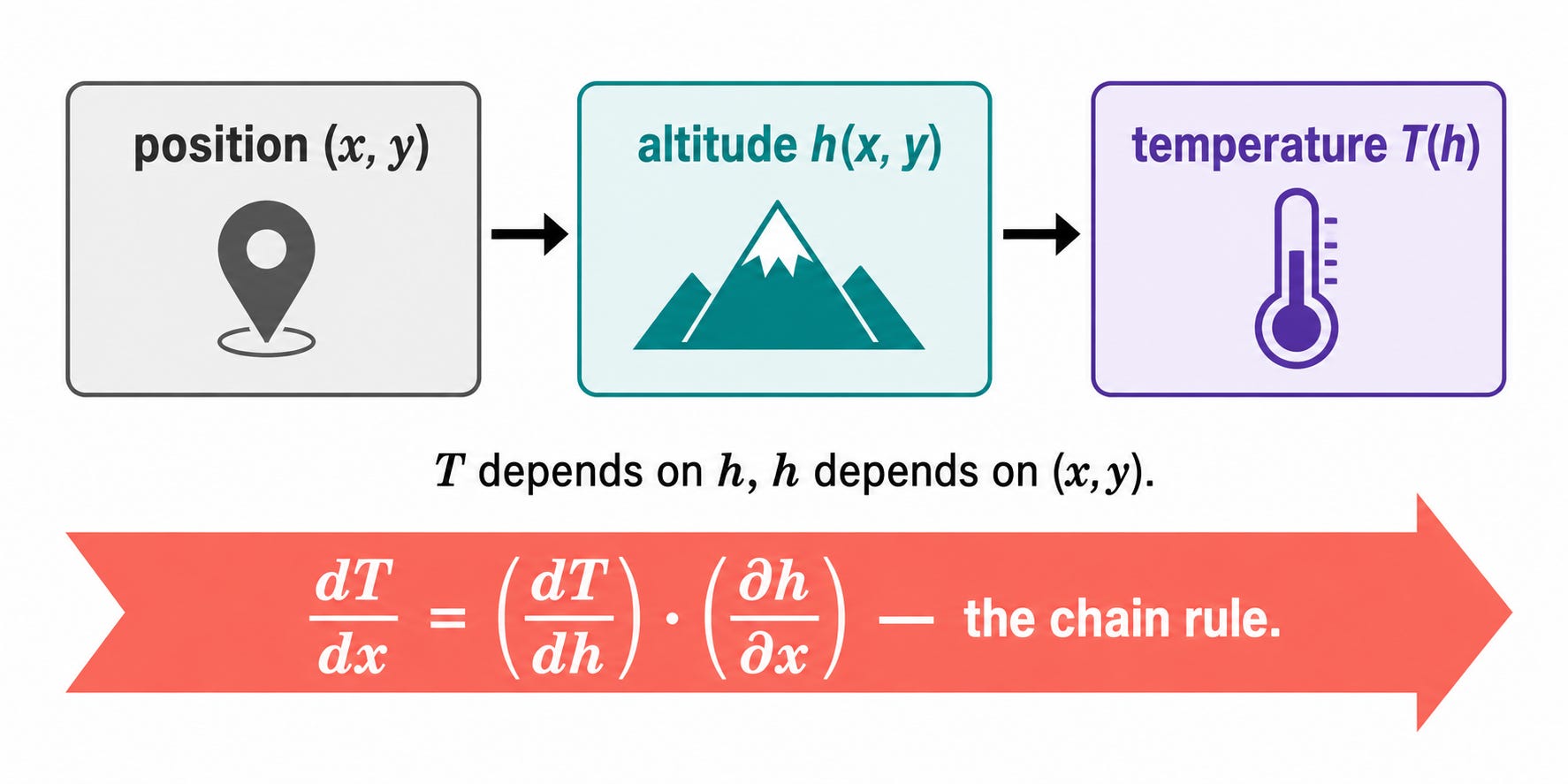
In Part 2 we introduced the partial derivative and the gradient. We learned to differentiate a function of several variables by varying one input at a time. But what happens when the inputs of a function are themselves functions of other variables?

This situation is everywhere in practice. And the tool that handles it is the chain rule: the rule that lets you differentiate through layers of composition. It is the most important differentiation rule in this series, and the mathematical backbone of backpropagation in neural networks.
Meet Nadia
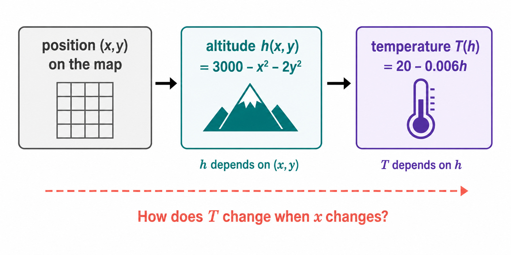
Nadia is a meteorologist working for a weather service in Switzerland. Her job is to predict the temperature at any location in the Alps. She knows two things from her models.
First, the altitude at any position (x, y) on the map (where x is the longitude and y is the latitude) is given by:
h(x, y) = 3000 - x² - 2y²
The altitude is 3000 meters at the origin (the summit) and decreases as you move away. Units are in meters.
Second, the temperature at any altitude h is given by:
T(h) = 20 - 0.006 · h
Temperature drops by 0.006°C for every meter of altitude gained. This is called the environmental lapse rate, a standard approximation in meteorology.
Nadia wants to know: if someone moves slightly east (increasing x), how does the temperature at their location change? This requires differentiating T with respect to x, but T does not depend directly on x. It depends on h, which depends on x. We need to chain the two relationships together.
The Chain Rule For One Variable
Before tackling Nadia’s situation, let us recall the chain rule from Part 1 in its simplest form.

If h is a function of x, and T is a function of h, then the composed function T(h(x)) has derivative:
dT/dx = (dT/dh) · (dh/dx)
Read it as: the rate at which T changes with x equals the rate at which T changes with h, times the rate at which h changes with x.
The name chain rule comes from exactly this: you chain the rates of change together. If h changes twice as fast as x, and T changes three times as fast as h, then T changes six times as fast as x. The rates multiply.
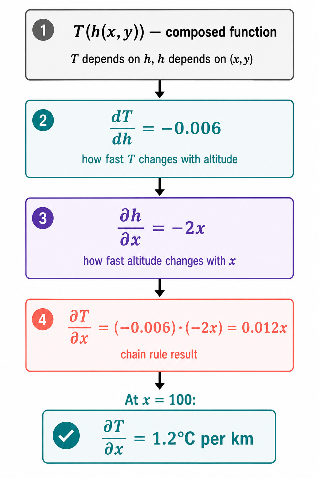
Let us apply this to Nadia’s problem along the x direction (holding y fixed):
dT/dh = -0.006
∂h/∂x = -2x
∂T/∂x = (dT/dh) · (∂h/∂x) = (-0.006) · (-2x) = 0.012x
At position x = 100 km east of the summit:
∂T/∂x = 0.012 × 100 = 1.2 °C per km
Moving east at that position, the temperature increases by 1.2°C per kilometer. This makes sense: moving away from the summit decreases altitude, and lower altitude means warmer temperature.
The Chain Rule In The Multivariate Setting
Nadia’s function depends on two variables x and y, not just x. The chain rule extends naturally to this case.
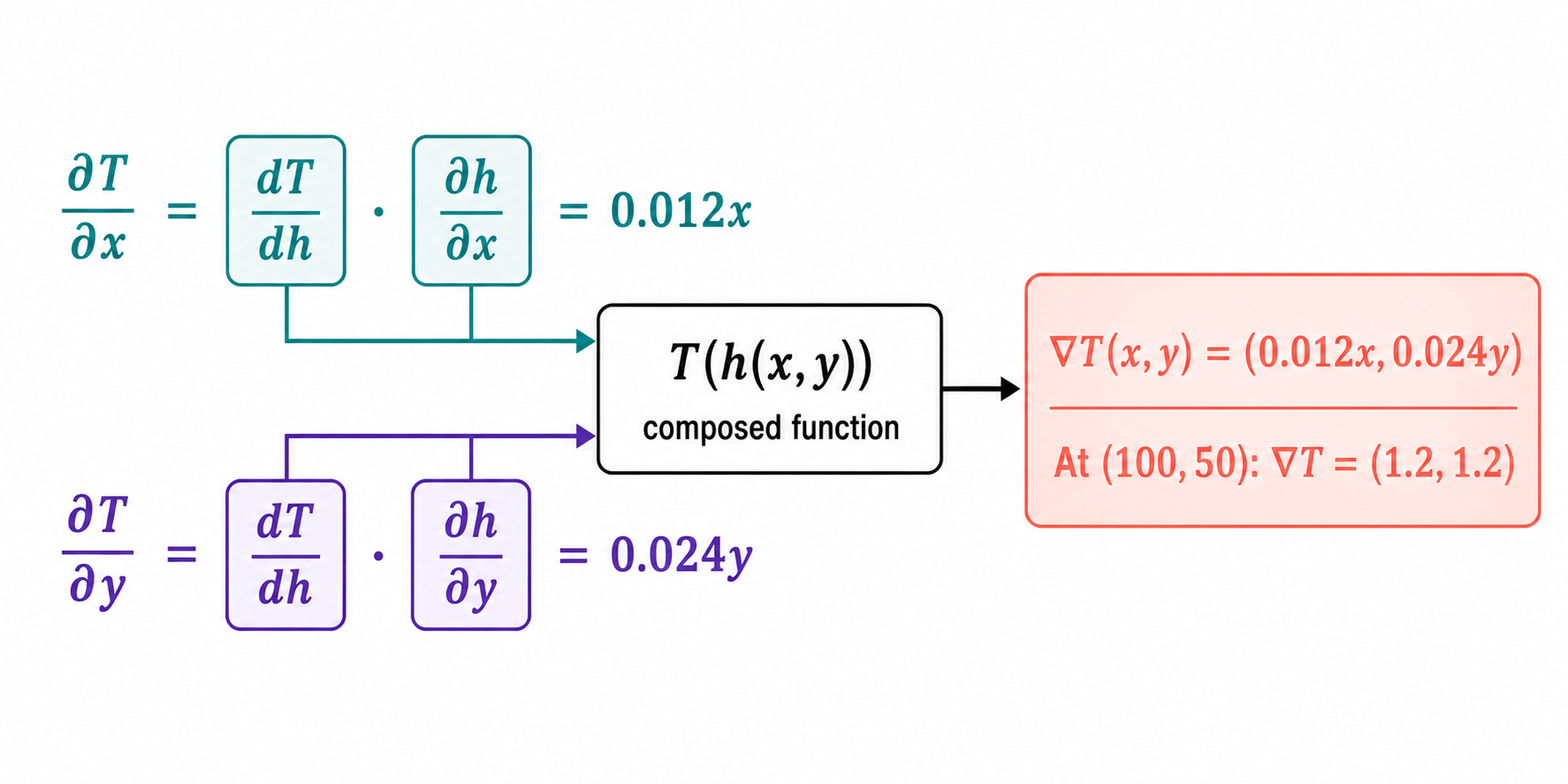
The composed function T(h(x, y)) has two partial derivatives, one for each input. Each is computed by the same chaining idea:
∂T/∂x = (dT/dh) · (∂h/∂x)
∂T/∂y = (dT/dh) · (∂h/∂y)
For Nadia’s functions:
dT/dh = -0.006
∂h/∂x = -2x
∂h/∂y = -4y
∂T/∂x = (-0.006) · (-2x) = 0.012x
∂T/∂y = (-0.006) · (-4y) = 0.024y
The gradient of T with respect to position (x, y) is:
∇T(x, y) = (0.012x, 0.024y)
At the position (x, y) = (100, 50):
∇T(100, 50) = (0.012 × 100, 0.024 × 50) = (1.2, 1.2)
Moving east and moving north both increase the temperature at the same rate at this position, 1.2°C per km in each direction.
The General Form
The real power of the chain rule emerges when both f and g are multivariate functions. Suppose:
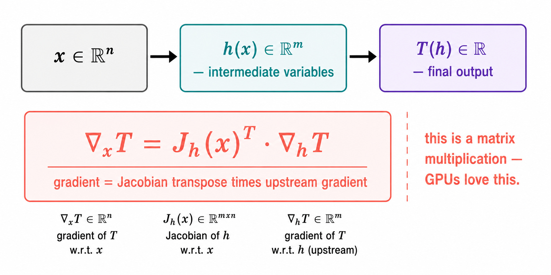
x is a vector in ℝⁿ
h(x) is a function from ℝⁿ to ℝᵐ (m intermediate variables)
T(h) is a function from ℝᵐ to ℝ
Then the gradient of T with respect to x is:
∇ₓT = Jₕ(x)ᵀ · ∇ₕT
where Jₕ(x) is the Jacobian matrix of h at x (the matrix of all partial derivatives of h with respect to x, which we will define properly in the next post) and ∇ₕT is the gradient of T with respect to h.
Do not worry if this looks abstract for now. The key message is this:
The chain rule in the multivariate setting is a matrix multiplication.
This is not a coincidence. It is the reason why gradient computations in neural networks can be organised as sequences of matrix multiplications, which modern hardware (GPUs) is extremely efficient at. The chain rule is not just a mathematical nicety, it is the reason deep learning is fast.
Wrapping Up
The chain rule states that when a function T depends on intermediate variables h, which in turn depend on inputs x, the derivative of T with respect to x is obtained by multiplying the rates of change along the chain. In the multivariate setting this becomes a matrix multiplication involving the Jacobian, which we will define properly in the next post.
We saw the chain rule at work in two settings: Nadia’s temperature model with one intermediate variable and the two-variable extension that gave us the full gradient.
In the next post we take one step back and ask: what happens when the function itself returns a vector instead of a number? The answer is the Jacobian matrix, and it brings the chain rule and the determinants from our earlier series together in one place.