

Vector Calculus Series Part 2 | The Gradient
Partial derivatives, the gradient, and the geometry behind them. When Your Function Has Several Inputs

In Part 1 we built the derivative for a function of one variable. The derivative f’(x) answered one question: how fast does f change as x moves?

But most functions in real life depend on more than one variable. The price of a house depends on its size, its location, and the number of rooms. The temperature in a room depends on your position in three dimensions. A loss function in machine learning depends on thousands of parameters at once.
When a function has several inputs, we need a new tool. That tool is the gradient. And to understand the gradient, we first need to understand partial derivatives.
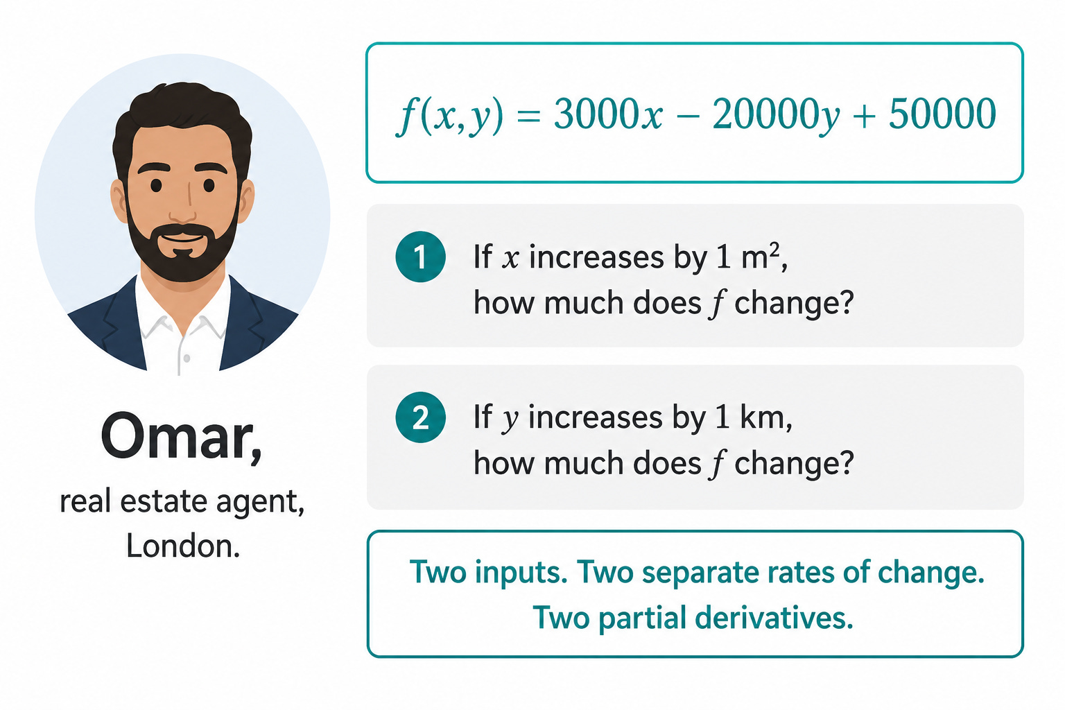
Meet Omar
Omar is a real estate agent in London. He is trying to understand what drives apartment prices in his neighborhood. After analysing hundreds of transactions he builds a simple model: the price of an apartment depends on two variables, its surface area in square meters and its distance from the nearest tube station in kilometers.
His model says:
f(x, y) = 3000x - 20000y + 50000
where x is the surface area in m² and y is the distance to the tube in km, and f(x, y) is the estimated price in pounds.
Omar wants to understand this function. Specifically he wants to know: if the surface area increases by 1 m², how much does the price change? And if the distance to the tube increases by 1 km, how much does the price change? These are two separate questions, and they have two separate answers.
The Partial Derivative
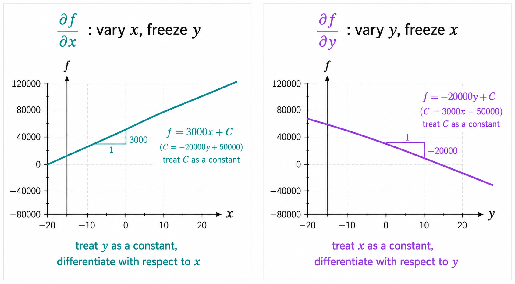
The key idea behind the partial derivative is simple: vary one input and freeze all the others.
To find how f changes with respect to x, we treat y as a constant and differentiate with respect to x exactly as we did in Part 1:
∂f/∂x = 3000
The notation ∂f/∂x (read “partial f partial x”) tells us: the rate of change of f with respect to x, with y held fixed. The answer is 3000: every additional square meter adds £3,000 to the price, regardless of the distance to the tube.
To find how f changes with respect to y, we treat x as a constant and differentiate with respect to y:
∂f/∂y = -20000
Every additional kilometer from the tube reduces the price by £20,000. The negative sign makes intuitive sense: further from the tube, cheaper.
A Less Obvious Example
Omar’s model was linear, so the partial derivatives were constants. Let us try a more interesting function to make sure the idea is clear.
Take:
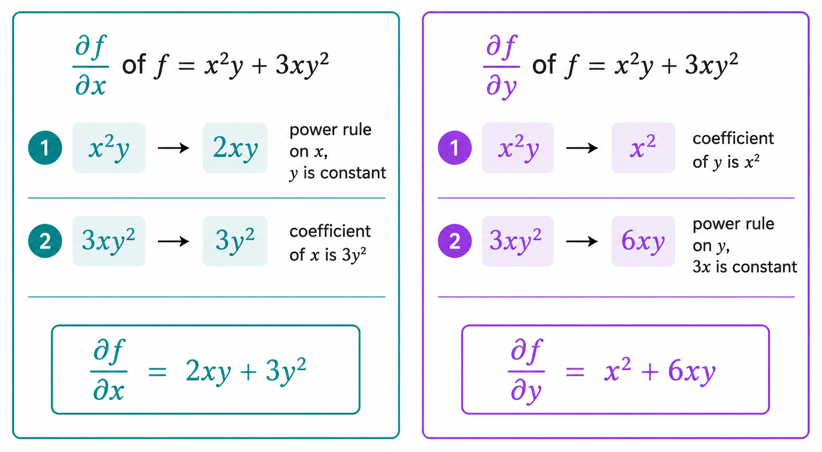
f(x, y) = x²y + 3xy²
To compute ∂f/∂x, treat y as a constant and differentiate with respect to x:
∂f/∂x = 2xy + 3y²
The term x²y differentiates to 2xy (by the power rule, treating y as a constant multiplier). The term 3xy² differentiates to 3y² (treating 3y² as the constant coefficient of x).
To compute ∂f/∂y, treat x as a constant and differentiate with respect to y:
∂f/∂y = x² + 6xy
The term x²y differentiates to x² (treating x² as the constant coefficient of y). The term 3xy² differentiates to 6xy (by the power rule on y², with 3x as the constant coefficient).
Notice that the partial derivatives are themselves functions of both x and y. At the point (1, 2) for example:
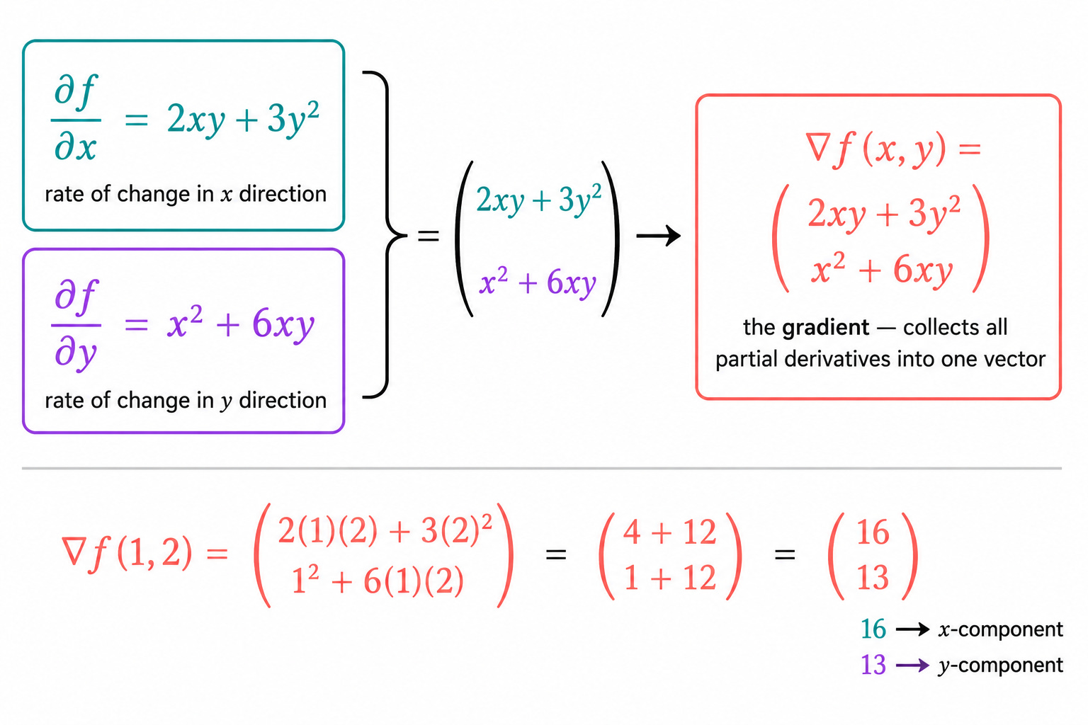
∂f/∂x (1, 2) = 2(1)(2) + 3(4) = 4 + 12 = 16
∂f/∂y (1, 2) = 1 + 6(1)(2) = 1 + 12 = 13
At the point (1, 2), the function increases 16 times faster in the x direction than it does for a unit increase in x, and 13 times faster in the y direction.
The Gradient
The two partial derivatives ∂f/∂x and ∂f/∂y each answer one question. But taken together they tell a richer story.
The gradient of f at a point (x, y) is the vector that collects all the partial derivatives:
∇f(x, y) = (∂f/∂x, ∂f/∂y)
The symbol ∇ is called “nabla”. For our example f(x, y) = x²y + 3xy²:
∇f(x, y) = (2xy + 3y², x² + 6xy)
At the point (1, 2):
∇f(1, 2) = (16, 13)
This is a vector in ℝ². It has a magnitude and a direction. And that direction carries deep geometric meaning.
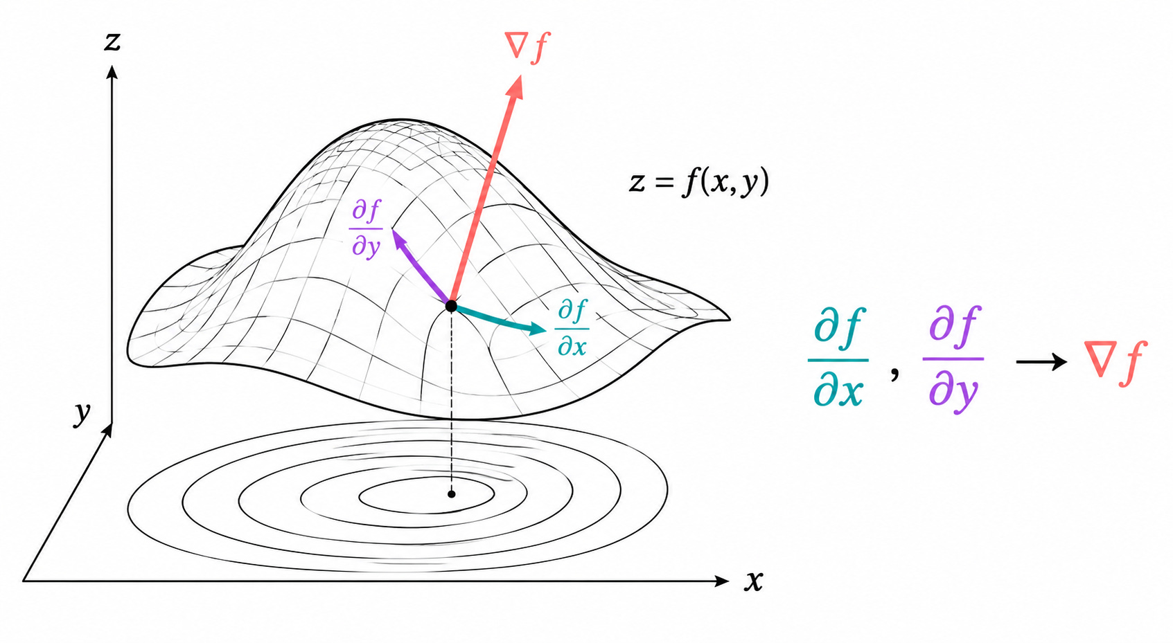
The Gradient Geometrically
Here is where the gradient becomes truly powerful. Let us think about what the function f(x, y) looks like as a surface in 3D: for every point (x, y) in the plane, the value f(x, y) gives the height above that point.
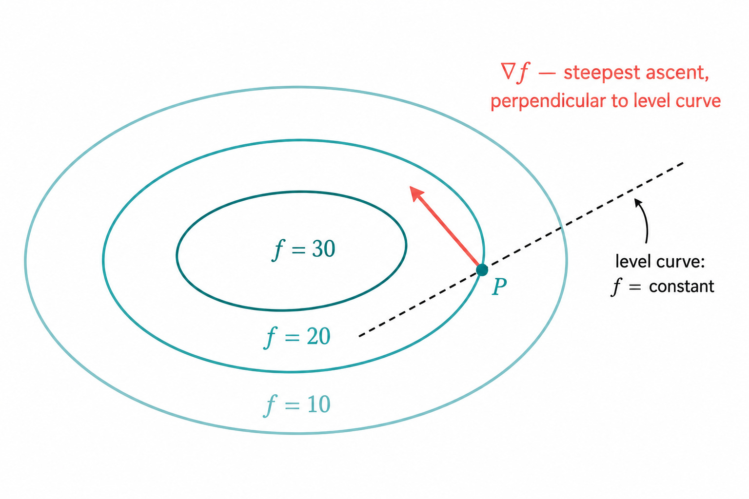
Now draw the level curves (also called contour lines): the curves in the xy-plane along which f takes a constant value. If you have ever seen a topographic map of a mountain, you have seen level curves. The closer they are together, the steeper the terrain.
The gradient ∇f at a point (x, y) is always perpendicular to the level curve passing through that point, and it points in the direction of steepest increase of f.
This is the key fact, and we proved it in Part 9 of the Cauchy-Schwarz series: among all unit vectors d, the one that maximizes the directional derivative ⟨∇f, d⟩ is the normalized gradient itself.

Now we understand what ∇f is made of: it is the vector of partial derivatives, assembled into a direction that tells you which way to climb.
The Gradient in Higher Dimensions
Everything we did for two variables extends naturally to any number of variables. If f depends on n variables x₁, x₂, …, xₙ, the gradient is:
∇f(x) = (∂f/∂x₁, ∂f/∂x₂, …, ∂f/∂xₙ)
This is a vector in ℝⁿ. In machine learning, a loss function might depend on millions of parameters. The gradient is a vector in that million-dimensional space. Its direction still points toward steepest increase, and its magnitude still tells you how steep the ascent is.
This is why the gradient is the central object of this entire series and of most of machine learning optimization: it tells you, at every point, in which direction to move to change the function the fastest.
Wrapping Up
The partial derivative ∂f/∂xᵢ measures how fast f changes when only the i-th input moves, with all others held fixed. It is computed using exactly the same rules as the derivative from Part 1, treating all other variables as constants.
The gradient ∇f collects all partial derivatives into a single vector. Geometrically it points in the direction of steepest increase of f, perpendicular to the level curves of f.
Omar used the gradient to understand which variable has the most influence on apartment prices.
In the next post we introduce the chain rule for multivariate functions.