Vector Calculus Series Part 1 | The Derivative

What Does It Mean for a Function to Change?

In the Cauchy-Schwarz series we used the gradient freely. In Part 9 we said that the gradient points in the direction of steepest ascent and that this is proved by Cauchy-Schwarz. That was true. But we skipped a step: we never asked what a gradient actually is, or how you compute one.

That is what this series is about.

We start at the very beginning: a single function of a single variable. No vectors, no matrices, no inner products yet. Just a curve and the question of how fast it is changing at any given point.

Stock Price

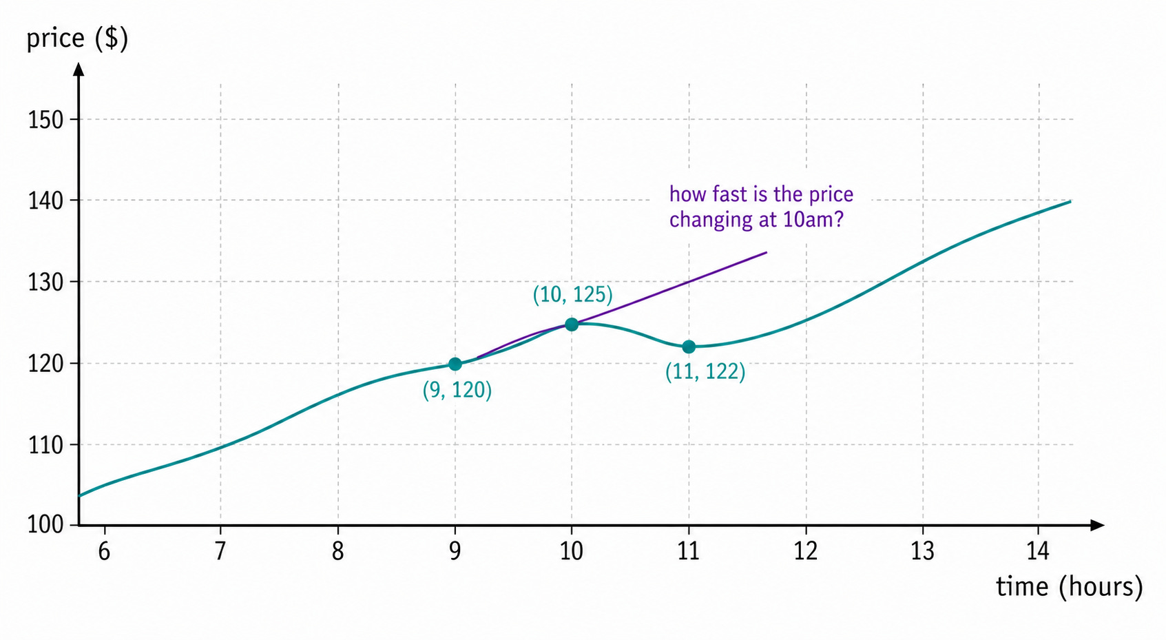
Imagine you are watching a stock price over the course of a day. At 9 a.m the price is $120. At 10 a.m it is $125. At 11 a.m it is $122. The price is moving, and you want to understand how it is moving.

One natural question is: at exactly 10 a.m, how fast was the price rising?

This is not asking for the average over the whole day. It is asking about the instantaneous rate of change at a specific moment. And answering it precisely is what the derivative does.

From Average to Instantaneous

Let us make this precise with a simpler function first. Take:

f(x) = x²

This is a parabola. At x = 2 the value is f(2) = 4. At x = 3 the value is f(3) = 9. Between x = 2 and x = 3, the function increased by 5 while x increased by 1. The average rate of change over that interval is:

average rate of change = (f(3) - f(2)) / (3 - 2) = (9 - 4) / 1 = 5

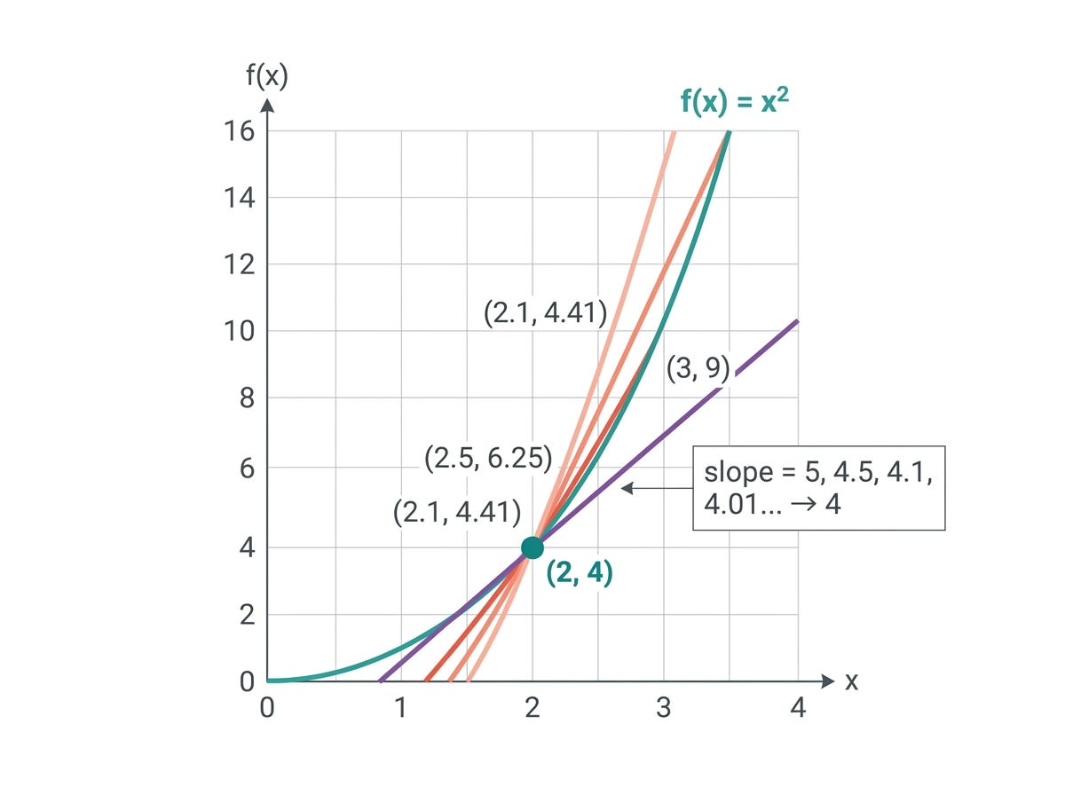
This is the slope of the line connecting the two points (2, 4) and (3, 9) on the curve. It is called the secant line.

But what if we want the rate of change not over an interval, but at the single point x = 2? We shrink the interval. Instead of looking from x = 2 to x = 3, we look from x = 2 to x = 2.5:

(f(2.5) - f(2)) / (2.5 - 2) = (6.25 - 4) / 0.5 = 4.5

Then from x = 2 to x = 2.1:

(f(2.1) - f(2)) / (2.1 - 2) = (4.41 - 4) / 0.1 = 4.1

Then from x = 2 to x = 2.01:

(f(2.01) - f(2)) / (2.01 - 2) = (4.0401 - 4) / 0.01 = 4.01

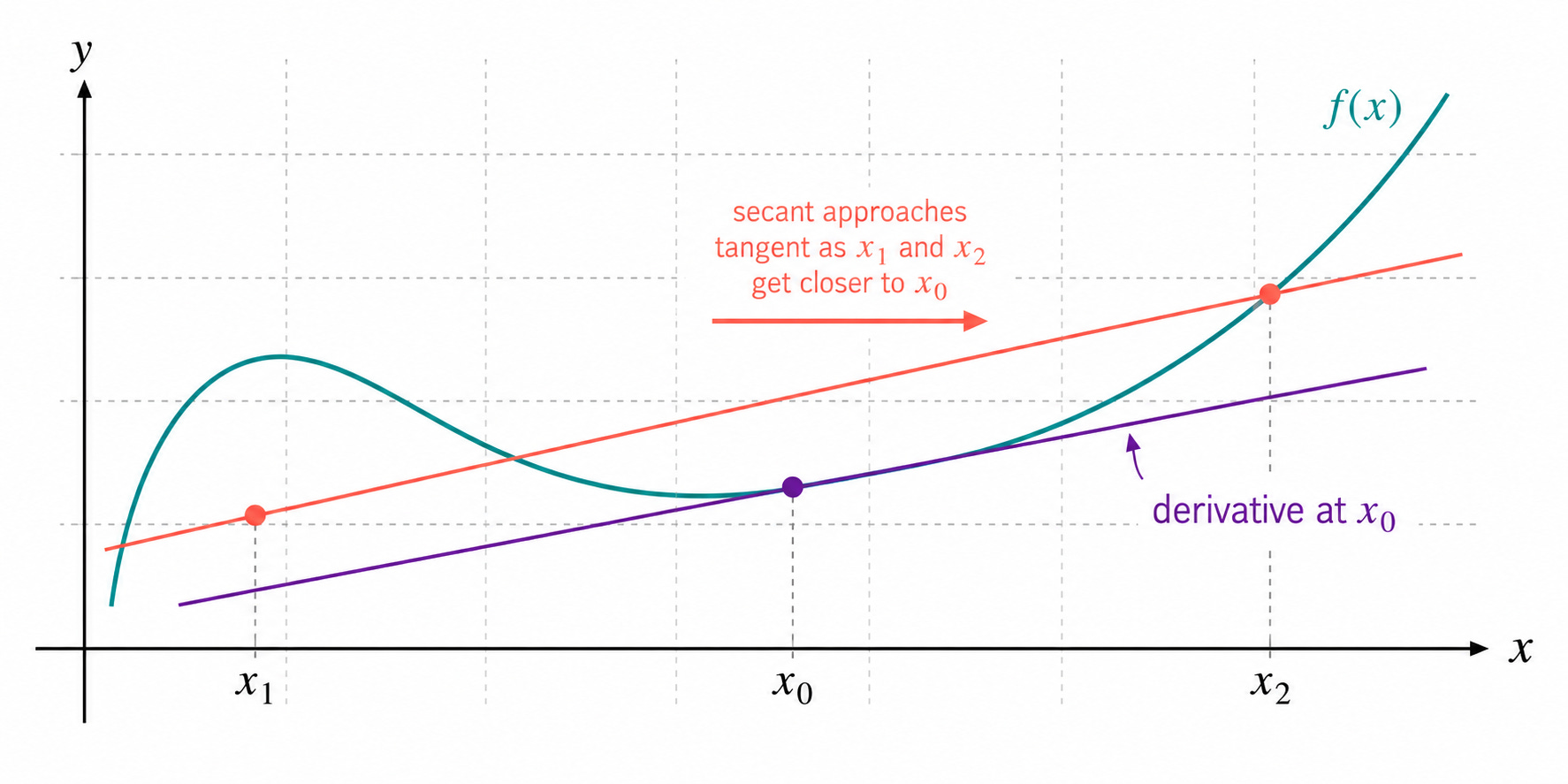
Something is happening. As the interval shrinks, the average rate of change is getting closer and closer to 4. The secant line is rotating, and in the limit it becomes the tangent line at x = 2.

Difference Quotient and Derivative

What we just did informally has a precise name. The ratio:

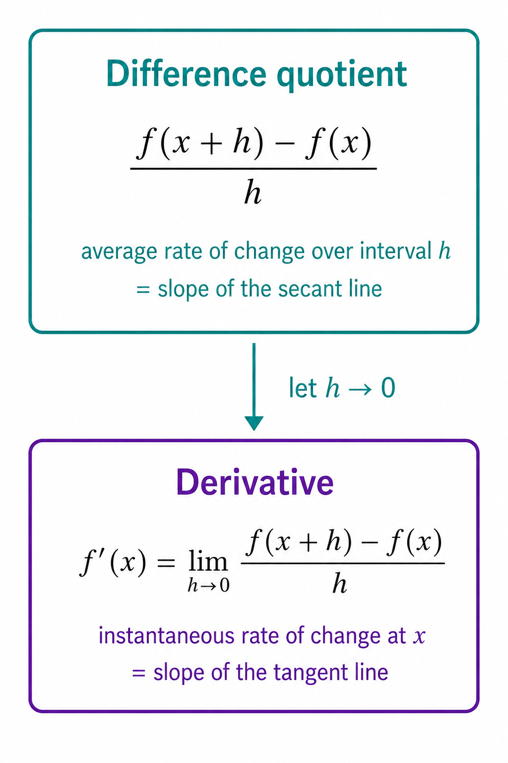
[f(x + h) - f(x)] / h

is called the difference quotient. It measures the average rate of change of f between x and x + h. The secant line through the two points (x, f(x)) and (x + h, f(x + h)) has exactly this slope.

When we let h approach zero, we get the derivative of f at x:

\(\begin{aligned} &f'(x) = \lim_{h \to 0} \frac{f(x + h) - f(x)}{h} \end{aligned}\)

This is the slope of the tangent line to the curve at the point x. It measures the instantaneous rate of change of f at that exact point.

The notation f’(x) is read “f prime of x”. You will also see it written as df/dx, which emphasises that it is the ratio of an infinitesimal change in f to an infinitesimal change in x.

The Derivative of f(x) = x²

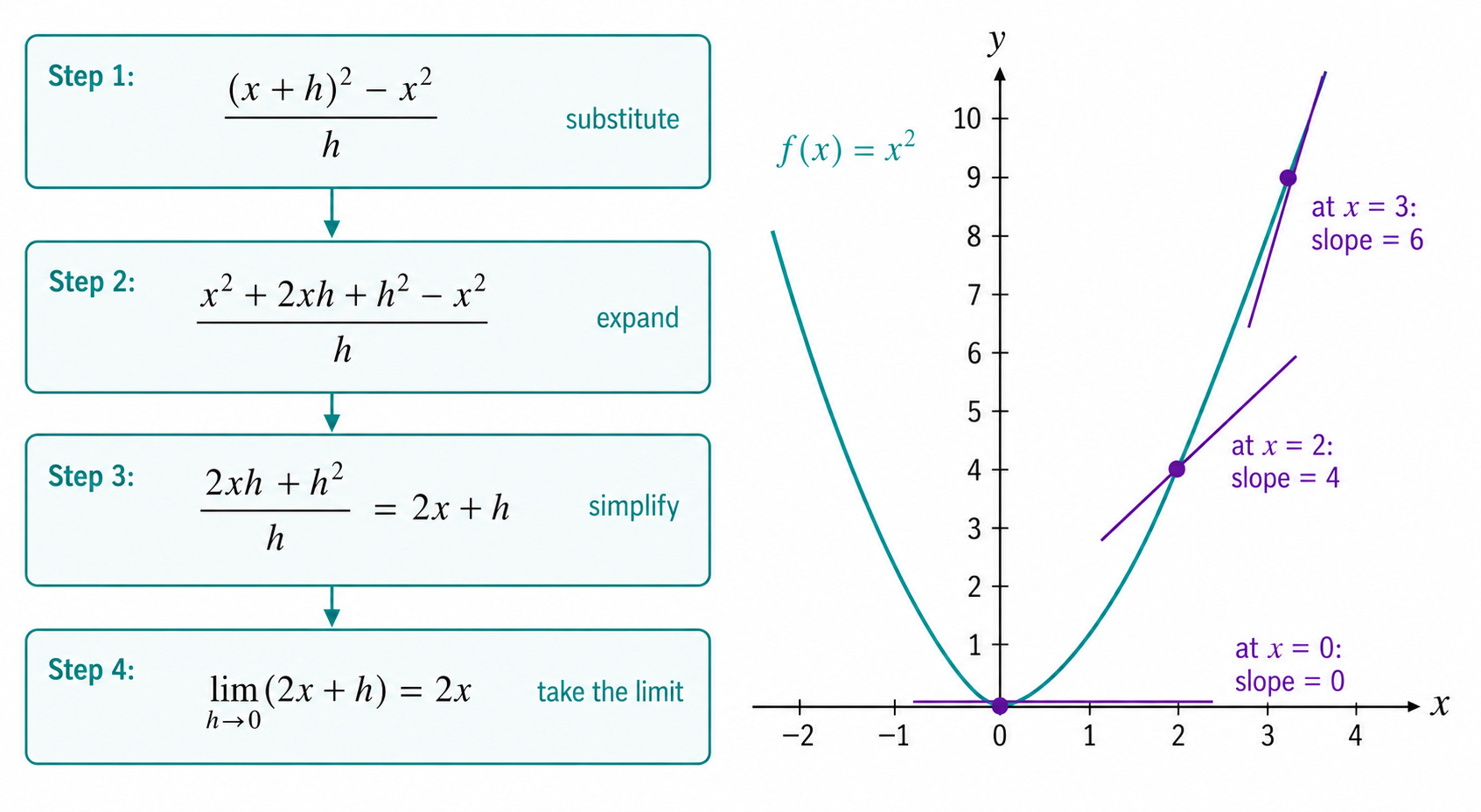
Let us now compute the derivative of f(x) = x² properly, using the definition. We want to find f’(x) for any x.

\(\begin{aligned} &\text{We start from the difference quotient:} \\ &\frac{f(x + h) - f(x)}{h} \\ &\text{Substituting } f(x) = x^2: \\ &= \frac{(x + h)^2 - x^2}{h} \\ &\text{Expanding } (x + h)^2: \\ &= \frac{x^2 + 2xh + h^2 - x^2}{h} \\ &= \frac{2xh + h^2}{h} \\ &= 2x + h \\ &\text{Now we let } h \text{ approach zero:} \\ &f'(x) = \lim_{h \to 0} (2x + h) = 2x \end{aligned}\)

The derivative of f(x) = x² is f’(x) = 2x.

Let us check this against what we computed earlier. At x = 2:

f’(2) = 2 × 2 = 4

This matches the limit we observed: 5, 4.5, 4.1, 4.01, converging to 4.

At x = 2 the curve has slope 4. At x = 3 it has slope 6. At x = 0 it has slope 0: the bottom of the parabola, where the curve is flat, exactly as you would expect.

Derivative’s Sign

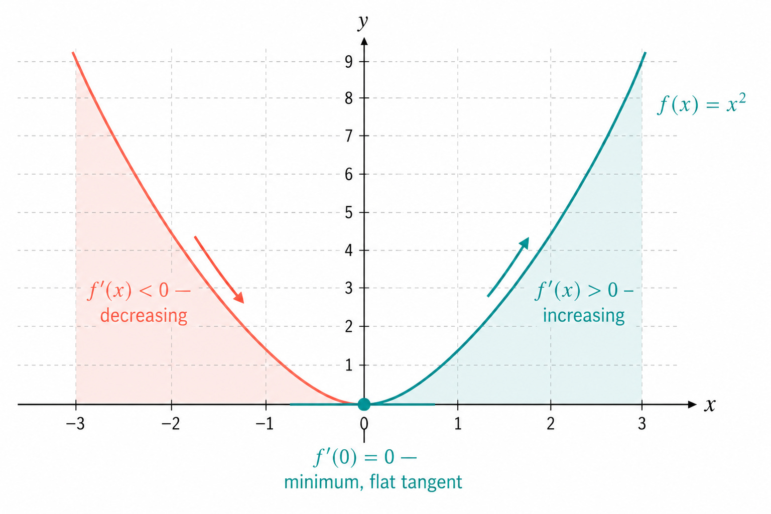
The derivative f’(x) = 2x has a clear geometric meaning depending on its sign.

When f’(x) > 0, the tangent slope is positive: the function is increasing at x. When f’(x) < 0, the slope is negative: the function is decreasing. When f’(x) = 0, the slope is zero: the function is flat at that point, either at a local minimum, a local maximum, or a saddle point.

For f(x) = x²:

• At x = -1: f’(-1) = -2 < 0. The parabola is going down.

• At x = 0: f’(0) = 0. The bottom of the parabola: a minimum.

• At x = 1: f’(1) = 2 > 0. The parabola is going up.

This is the first glimpse of why the derivative matters for optimization. If you want to find the minimum of a function, you look for the point where f’(x) = 0. We will come back to this idea in every post of this series.

The Four Rules

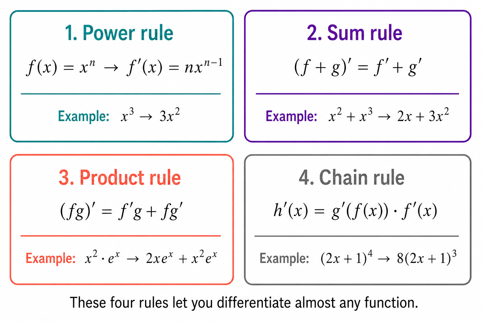
Computing derivatives from the limit definition every time would be tedious. Fortunately, a set of rules lets you compute derivatives of almost any function directly, without going back to limits.

Here are the four essential ones:

\(\begin{aligned} &\text{Power rule: if } f(x) = x^n, \text{ then } f'(x) = nx^{n-1} \\ &f(x) = x^3 \quad \rightarrow \quad f'(x) = 3x^2 \\ &f(x) = x^5 \quad \rightarrow \quad f'(x) = 5x^4 \end{aligned}\)

\(\begin{aligned} &\text{Sum rule: } (f + g)' = f' + g' \\ &f(x) = x^2 + x^3 \quad \rightarrow \quad f'(x) = 2x + 3x^2 \end{aligned}\)

\(\begin{aligned} &\text{Product rule: } (f \cdot g)' = f' \cdot g + f \cdot g' \\ &f(x) = x^2 \cdot \sin(x) \quad \rightarrow \quad f'(x) = 2x \cdot \sin(x) + x^2 \cdot \cos(x) \end{aligned}\)

\(\begin{aligned} &\text{Chain rule: if } h(x) = g(f(x)), \text{ then } h'(x) = g'(f(x)) \cdot f'(x) \\ &h(x) = (2x + 1)^4 \\ &f(x) = 2x + 1, \quad f'(x) = 2 \\ &g(f) = f^4, \quad g'(f) = 4f^3 \\ &h'(x) = 4(2x + 1)^3 \cdot 2 = 8(2x + 1)^3 \end{aligned}\)

The chain rule is the most important of these four. It will reappear in other part of this series in a much more powerful form, and it is the mathematical engine behind backpropagation.

Back to Stock Price

Remember the stock price at the start of this post. The price over time can be modeled as a function f(t). The derivative f’(t) tells you the instantaneous rate of change of the price at time t.

If f’(t) > 0 the price is rising at that moment. If f’(t) < 0 it is falling. If f’(t) = 0 it is at a local peak or trough.

A trader watching the derivative of a price function is not doing anything mysterious. They are asking: at this exact moment, which way is the function moving and how fast?

That is the derivative. One number, attached to one point on a curve, answering one question: how fast is this changing right now?

Wrapping Up

The derivative of a function f at a point x is defined as:

\(\begin{aligned} &f'(x) = \lim_{h \to 0} \frac{f(x + h) - f(x)}{h} \end{aligned}\)

It is the slope of the tangent line to the curve at x. It measures the instantaneous rate of change of f at that exact point.

We computed it from scratch for f(x) = x² and found f’(x) = 2x. We verified it matches the numerical approximations. We saw that the sign of the derivative tells us whether the function is increasing, decreasing, or flat. And we introduced four rules that let us differentiate any function without returning to the limit definition.

In the next post we extend this idea to functions of several variables.