Vector Calculus Series Part 4 | The Jacobian

Functions That Return Vectors. When your function has several outputs, the derivative becomes a matrix.

In Part 2 we studied functions that take several inputs and return a single number: f: ℝⁿ → ℝ. The gradient was the right tool for that case.

Vector Calculus Series Part 2 | The Gradient

In Part 3 we saw that the chain rule in the multivariate setting involves a matrix multiplication. We mentioned the Jacobian without defining it precisely and promised to come back to it.

Vector Calculus Series Part 3 | The Chain Rule

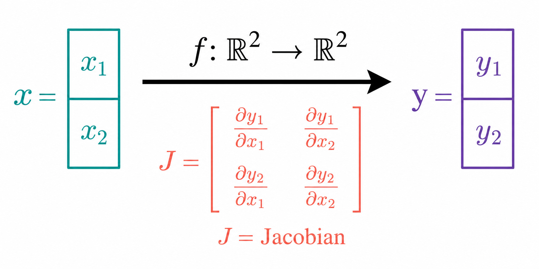
Today we do exactly that. We extend our framework to functions that take several inputs and return several outputs: f: ℝⁿ → ℝᵐ. The derivative of such a function is no longer a vector.

Nadia’s Wind Model

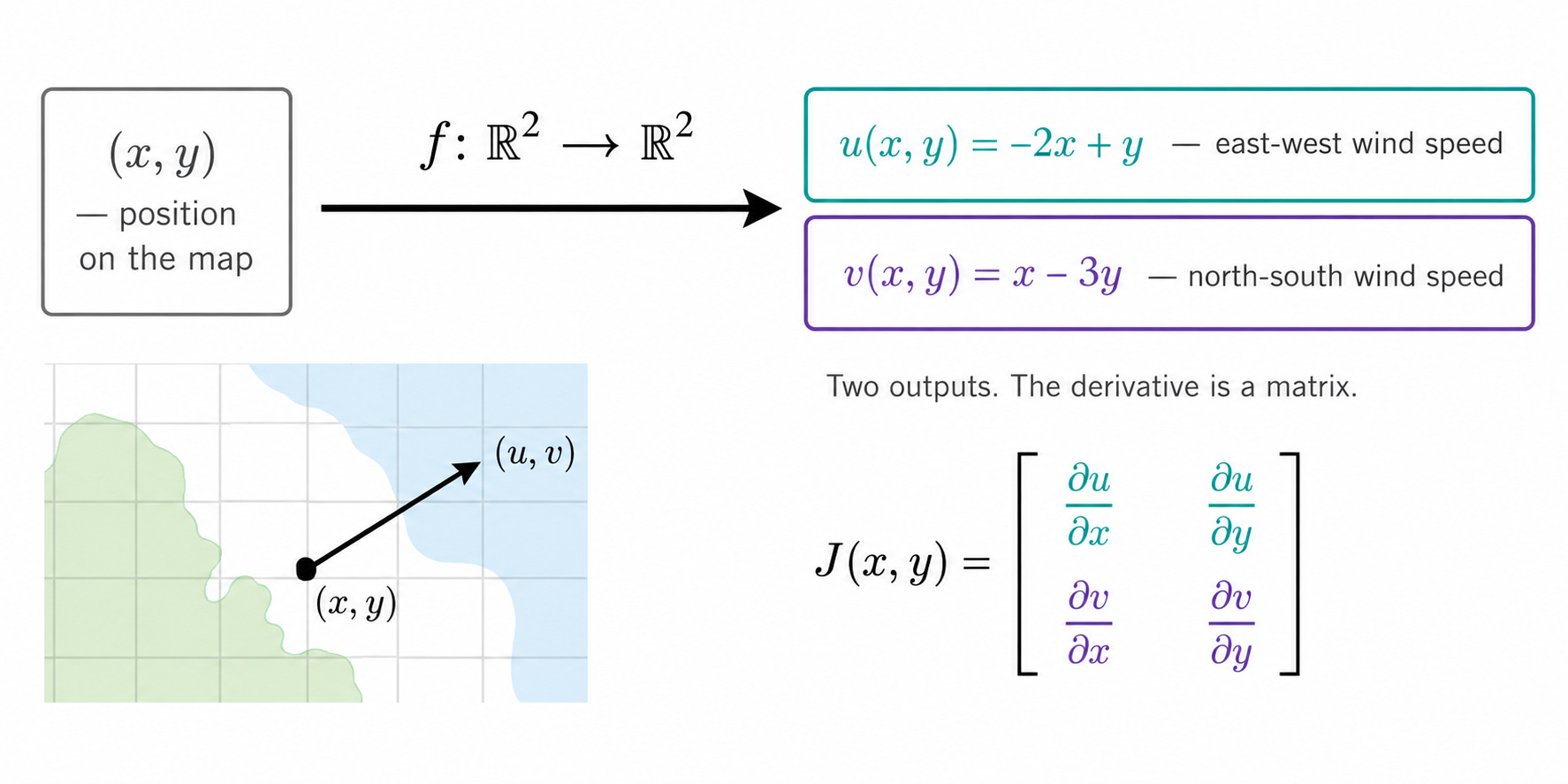
Nadia is back. In Part 3 she modeled the temperature at any position (x, y) on her map of the Alps. Now her team needs something more: a model for the wind at every position.

Wind is not a single number. It has two components: a speed in the east-west direction (u) and a speed in the north-south direction (v). Together they form a vector (u, v) that tells you both how fast the wind blows and in which direction.

Nadia’s model gives the wind vector at position (x, y) as:

u(x, y) = -2x + y (east-west wind speed, in m/s)

v(x, y) = x - 3y (north-south wind speed, in m/s)

This defines a function f: ℝ² → ℝ² that takes a position and returns a wind vector:

f(x, y) = (u(x, y), v(x, y)) = (-2x + y, x - 3y)

Two inputs. Two outputs. How does this function change as the position moves? The gradient is no longer the right tool. We need the Jacobian.

From Gradient to Jacobian

In Part 2, the gradient of a scalar function f: ℝⁿ → ℝ collected all the partial derivatives into a single row vector:

∇f = (∂f/∂x₁, ∂f/∂x₂, …, ∂f/∂xₙ)

Now our function has m outputs instead of one. Each output yᵢ has its own gradient with respect to the inputs. The Jacobian stacks all those gradients as rows into a single matrix:

\(\begin{aligned} &J = \begin{bmatrix} \frac{\partial y_1}{\partial x_1} & \frac{\partial y_1}{\partial x_2} & \cdots & \frac{\partial y_1}{\partial x_n} \\ \frac{\partial y_2}{\partial x_1} & \frac{\partial y_2}{\partial x_2} & \cdots & \frac{\partial y_2}{\partial x_n} \\ \vdots & \vdots & \ddots & \vdots \\ \frac{\partial y_m}{\partial x_1} & \frac{\partial y_m}{\partial x_2} & \cdots & \frac{\partial y_m}{\partial x_n} \end{bmatrix} \end{aligned}\)

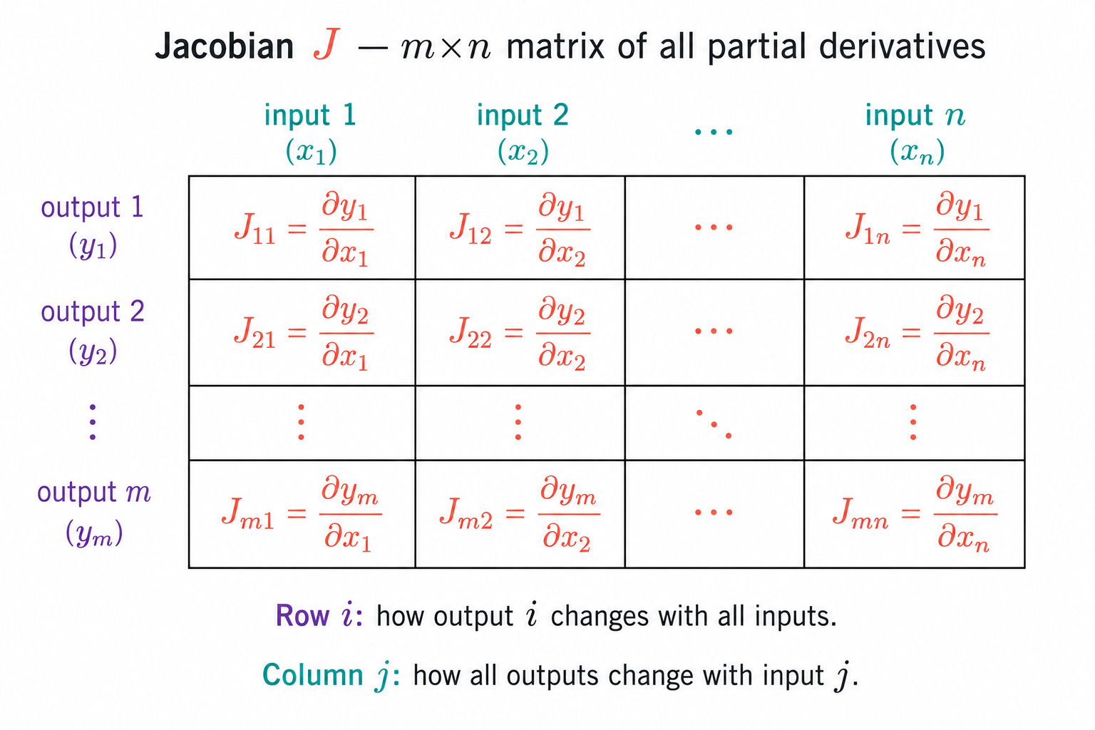
The Jacobian is an m×n matrix. Row i contains the partial derivatives of the i-th output with respect to all inputs. Column j contains the partial derivatives of all outputs with respect to the j-th input.

The entry Jᵢⱼ = ∂yᵢ/∂xⱼ answers a precise question: how much does the i-th output change when the j-th input increases by a small amount?

Computing Nadia’s Jacobian

Let us compute the Jacobian for Nadia’s wind model:

f(x, y) = (u, v) = (-2x + y, x - 3y)

The Jacobian is a 2×2 matrix (2 outputs, 2 inputs):

\(\begin{aligned} &J = \begin{bmatrix} \frac{\partial u}{\partial x} & \frac{\partial u}{\partial y} \\ \frac{\partial v}{\partial x} & \frac{\partial v}{\partial y} \end{bmatrix} \end{aligned}\)

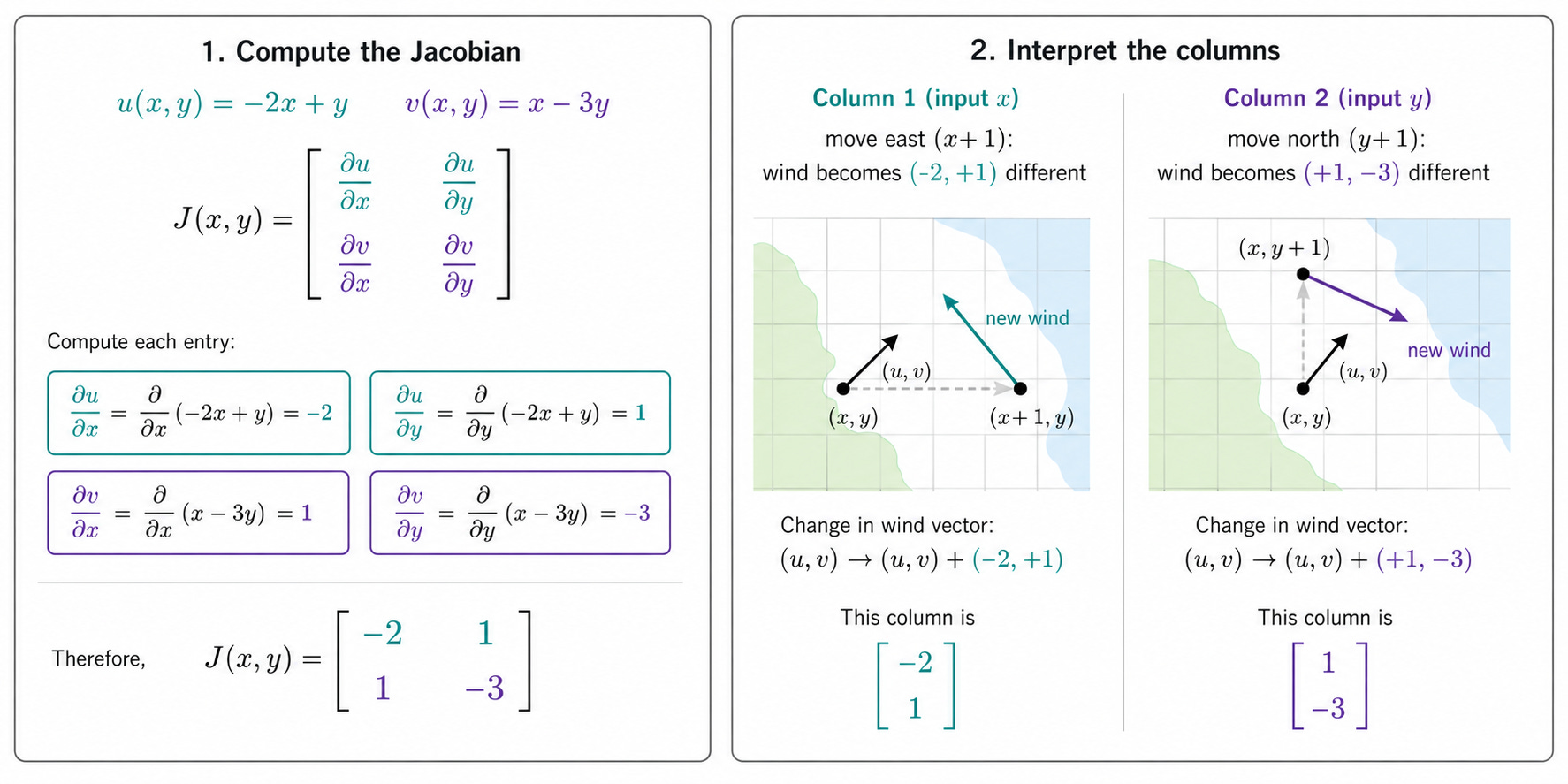
Computing each entry:

∂u/∂x = -2, ∂u/∂y = 1

∂v/∂x = 1, ∂v/∂y = -3

So the Jacobian is:

\(\begin{aligned} &J = \begin{bmatrix} -2 & 1 \\ 1 & -3 \end{bmatrix} \end{aligned}\)

Notice that this is a constant matrix: the Jacobian does not depend on the position (x, y) because the wind model is linear. For nonlinear functions the Jacobian would change at every point, just like the gradient does.

Each column tells Nadia how the wind vector changes when one input moves. The first column (-2, 1) says: if x increases by 1 km (moving east), the east-west wind changes by -2 m/s and the north-south wind changes by +1 m/s. The second column (1, -3) says: if y increases by 1 km (moving north), the east-west wind changes by +1 m/s and the north-south wind changes by -3 m/s.

Linear Approximation

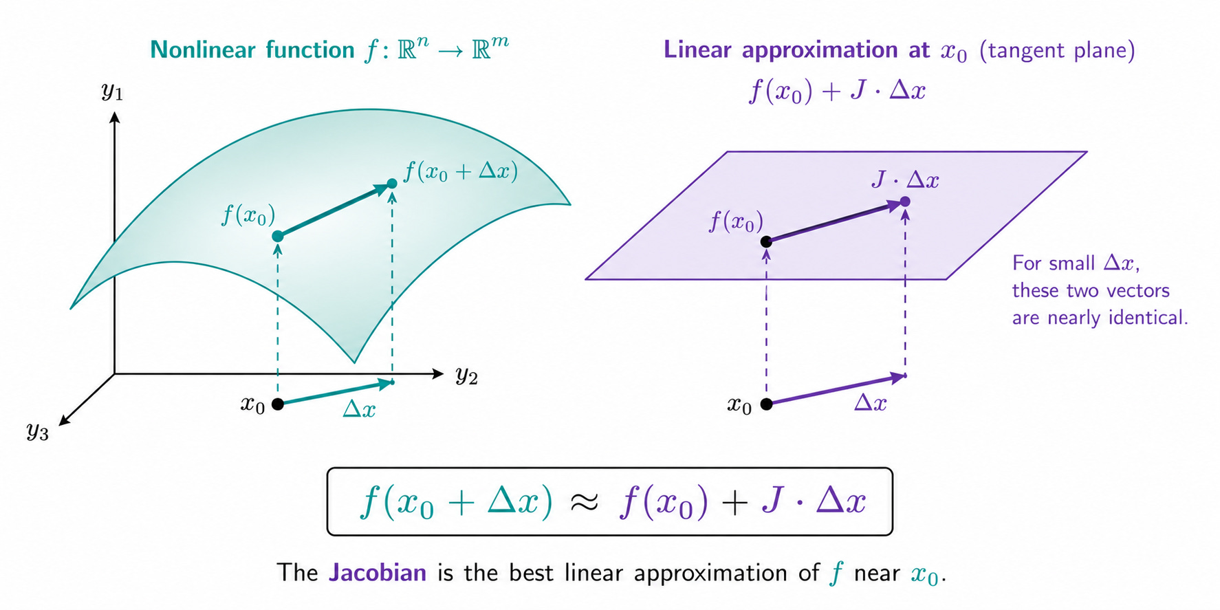
There is a deeper way to understand the Jacobian. Near any point x₀, a differentiable function f: ℝⁿ → ℝᵐ can be approximated by a linear function:

f(x₀ + Δx) ≈ f(x₀) + J · Δx

where Δx is a small displacement from x₀ and J is the Jacobian at x₀. This is the multivariate version of the tangent line approximation from Part 1.

The Jacobian J tells you: if you move by a small vector Δx in the input space, the output changes by approximately J·Δx. The Jacobian is the best linear approximation of f near x₀.

For Nadia’s wind model at any point:

f(x + Δx, y + Δy) ≈ f(x, y) + J · (Δx, Δy)

= (-2x + y, x - 3y) + (-2Δx + Δy, Δx - 3Δy)

A small step (Δx, Δy) on the map produces a wind change of (-2Δx + Δy, Δx - 3Δy). The Jacobian encodes all of this in one matrix.

The Completed Chain Rule

Now we can write the chain rule from Part 3 in its full and precise form.

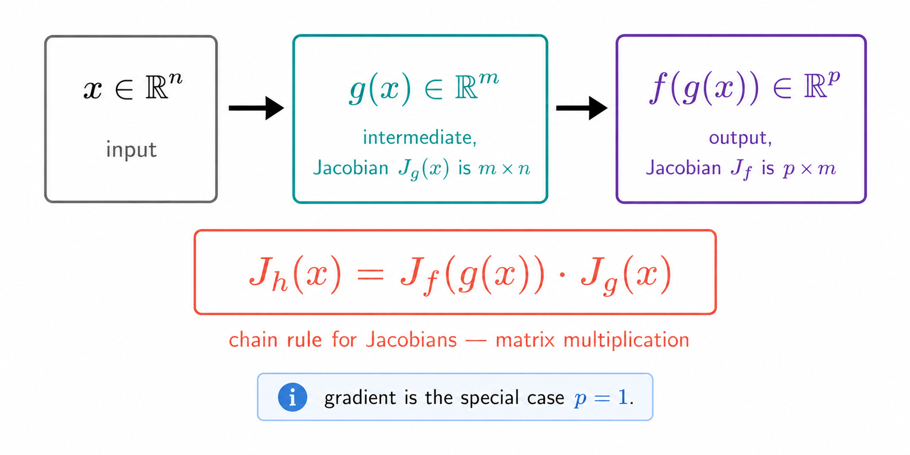
Suppose g: ℝⁿ → ℝᵐ and f: ℝᵐ → ℝᵖ are two differentiable functions. Their composition h = f ∘ g maps ℝⁿ → ℝᵖ. The Jacobian of h at a point x is:

\(\begin{aligned} &J_h(x) = J_f(g(x)) \cdot J_g(x) \end{aligned}\)

The Jacobian of the composition is the product of the individual Jacobians, evaluated at the right points. This is exactly the matrix multiplication we mentioned in Part 3.

The Jacobian is the right generalization of the gradient and the derivative. Gradient is Jacobian for scalar outputs. Derivative is Jacobian for one-dimensional functions. The Jacobian unifies all cases.

Wrapping Up

The Jacobian is the natural extension of the gradient to vector-valued functions. Where the gradient of f: ℝⁿ → ℝ is a vector in ℝⁿ, the Jacobian of f: ℝⁿ → ℝᵐ is an m×n matrix whose entry Jᵢⱼ = ∂yᵢ/∂xⱼ tells you how the i-th output changes with the j-th input.

It provides the best linear approximation of f near any point and completes the chain rule as a matrix multiplication.

Nadia used the Jacobian to understand how her wind model responds to changes in position: a 2×2 matrix that encodes, in one object, all four rates of change between her two inputs and two outputs.

In the next post we add a second layer of information: not just how fast the function changes, but how that rate of change itself changes.